Investment risk in retirement and the Annual Performance Test
Addressing investment risk is a vital part of the design of post-retirement products. The question of how to measure it has been addressed by the Australian Government Actuary (AGA) who has looked at the probabilities of falling short of a target.
This approach requires a method to simulate investment performance realistically. The critical question here is how and why investment markets fluctuate over short and long periods. Colin Grenfell’s thorough analysis of past data indicates that the distributions are not normal. Colin’s paper identifies the presence of complex correlation relationships, both short-term and long-term. This can result in some difficulty in making sure stochastic modelling appropriately reflects this, and in ensuring consistency across participants. Given this, analysing historical data may prove useful in revealing potential outcomes.
Given the current prevalence of high inflation, the aim of this article is to investigate the potential effects of such an environment on retirement income levels and investment strategy performance. In addition, this article will analyse the performance of a typical investment strategy under high inflation to examine the effectiveness of a portfolio with a simple risk management overlay in such an environment.
High Inflation in the 1970s
The AGA technical paper recommends utilising stochastically generated scenarios as a means of calculating retirement income risk measures. However, there is often considerable variation in how these stochastic scenarios are generated and the level of sophistication and assumptions used can vary significantly. The variability in these scenarios can therefore lead to a substantially different set of outcomes.
As a result, in the analysis we outline in this article, we have instead focused on using historical data to gain insight into how a particular investment strategy would have performed in the past.
We have focused primarily on the highly turbulent and poorly performing investment markets during the 1970s. This historic period of high inflation is particularly relevant given the way in which governments have stimulated economies and increased money supply over the past two years. This has led to high inflation and interest rates with risks that may continuously persist in future years. As outlined in the Actuaries Institute’s recent Green Paper, there is a material risk that we will experience yet again a period of persistent high inflation and low growth.
Looking at the historical period 1973-1982 and the US markets (where data is most widely available), it is not a pretty picture. These years encompassed a highly inflationary period which included the recovery of inflation back to a normal range as shown in Figure 1. During this period, a typical 70/30 investment portfolio[1] would have faced a challenging start with an initial sell-off until 1974 which caused a significant drawdown of ‑30.9%.
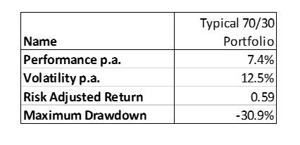
Despite this setback, this portfolio would have subsequently experienced a gradual recovery for the remainder of this period. As highlighted in Figure 3, the investment performance led to a Sharpe ratio of 0.59 for the entire period while annual inflation peaked at over 14%.
Figure 1: US Annual Inflation 1970-1985
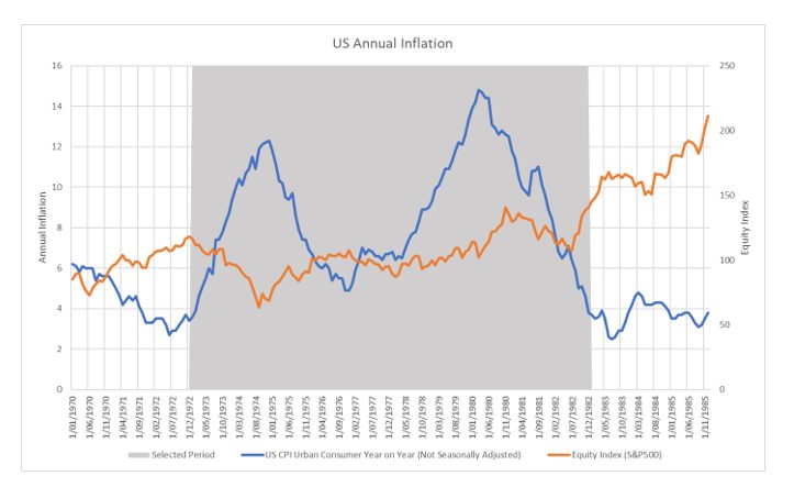
Figure 2: Cumulative return of a typical 70/30 portfolio 1973-1982
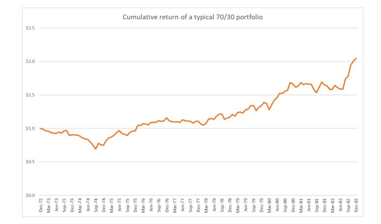
Figure 3: Summary Statistics on a typical 70/30 Portfolio 1973-1982
Background of Analysis
For the purpose of this article, we have examined the comparative performance of two hypothetical market-linked annuities in a pooled structure[2]:
- One where the income is linked to a typical 70% US equities and 30% US government bonds investment portfolio without any risk management overlay1 (Reference Portfolio); and
- another where the income is again linked to the same 70/30 investment portfolio but with a managed equity risk component (i.e., the Managed Volatility Portfolio).
The Managed Volatility Portfolio seeks to mitigate equity risk by regulating the allocation to equities during periods of heightened volatility and to sustain a balanced level of risk allocation to the equity asset class.
It does this by shifting allocations from equities to the money market when the forecasted equity volatility surpasses a target volatility level, and vice versa, until volatility returns to that target level. For the purpose of this analysis, the target volatility level was set to 8% p.a. without the use of leverage. The volatility forecasts are based on the EGARCH2 process, which extends the Exponential GARCH model proposed by Nelson (1991) by including both short-and long-term dynamic factors. The 70%/30%1 split between equities and bonds is intended to mirror a typical growth portfolio that an investor could invest in.
The time frame under consideration is 1973-1982 – a period which as mentioned previously was characterised by rampant inflation and subsequent normalisation.
Portfolio Performance & Risk
Figure 4: Managed Volatility Portfolio vs Reference Portfolio cumulative return
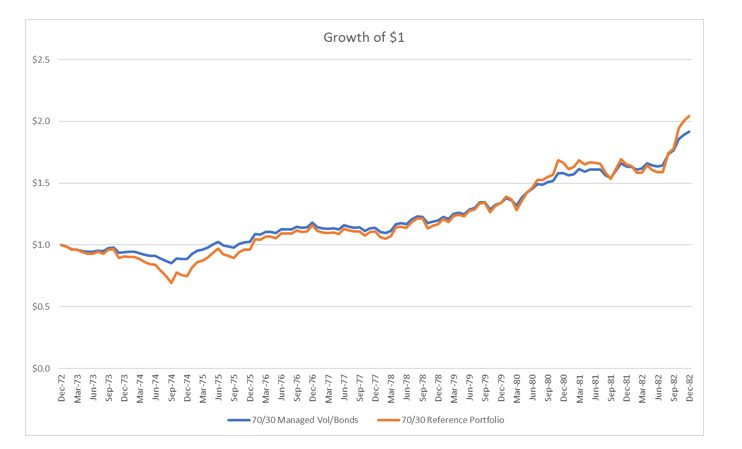
Figure 5: Summary Statistics on the Managed Volatility Portfolio vs Reference Portfolio
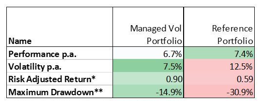
*Risk Adjusted Return = Performance p.a. / Volatility p.a.
**Maximum Drawdown = Maximum observed portfolio loss from a peak to a trough, before a new peak is attained
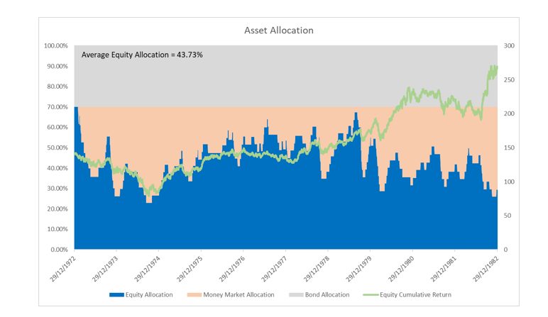
Figure 6: Asset allocation of the Managed Volatility Portfolio
As seen in Figure 4, the Managed Volatility Portfolio outperformed the Reference Portfolio during the 1973-74 equity sell-off. Subsequently, the equity market experienced a recovery phase where the market level eventually surpassed its high watermark.
During this period, the Reference Portfolio started to catch up and eventually surpassed the Managed Volatility Portfolio. From a cumulative performance perspective, market volatility forecast during this period was higher than the 8% p.a. volatility target.
From a risk perspective, the Managed Volatility Portfolio was successful in reducing its maximum drawdown to -14.9% – a decrease of over half from the -30.9% in the Reference Portfolio. Additionally, the portfolio volatility of the Managed Volatility Portfolio was reduced to 7.5% p.a. from 12.5% p.a. in the Reference Portfolio, leading to a significant improvement in the risk-adjusted return from 0.59 to 0.90 (see Figure 5).
Impact on Retirement Income
As with any analysis that focuses on retirees, it is important to focus on member outcomes – particularly as one of the key metrics that retirees are concerned with is the level of real regular income received during retirement.
In this analysis, we’ve assumed that at the start of the period, a 67-year-old member with a $100k balance had invested in two different types of retirement income schemes for comparison:
- A hypothetical market-linked annuity in a pooled structure. The discount rate[3] for the annuity has been set to 7.4% p.a.[4] based on typical equity risk premiums and the risk-free rates in December 1972.
- An account-based pension with income payment following the minimum annual payment schedule for super income streams[5].
Figure 7: Nominal monthly income for market-linked annuity
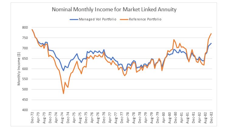
Figure 8: Nominal monthly income for an account-based pension
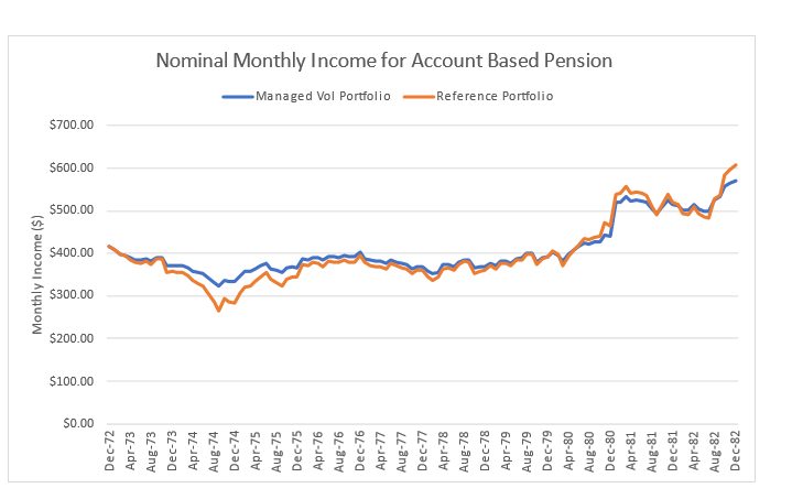
Figure 9: Real monthly income for market-linked annuity
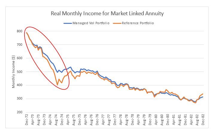
Figure 10: Real monthly income for account-based pension
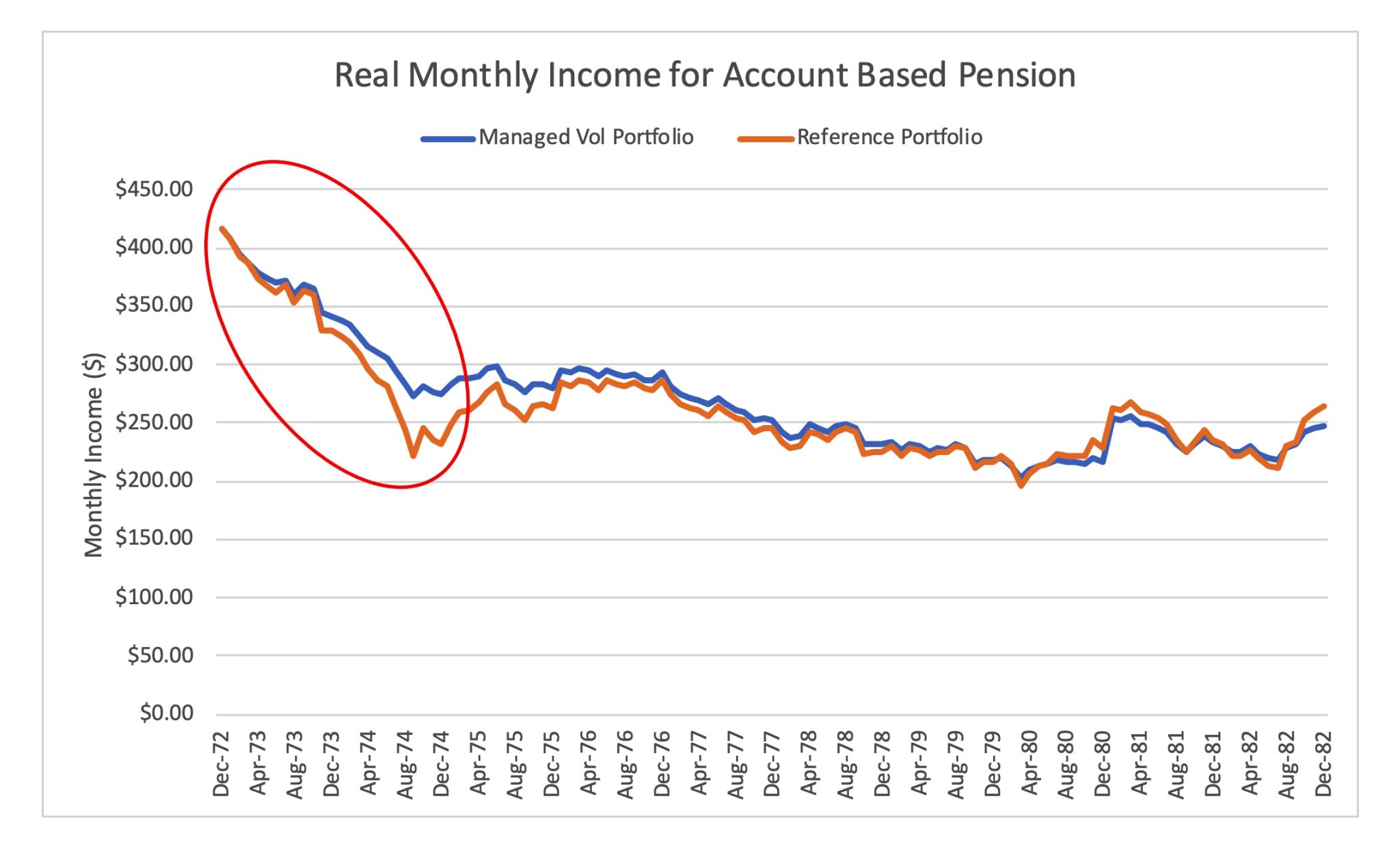
Regardless of which investment strategy had been selected, a significant decline in real income levels for members in the market-linked annuity and account-based pension during the 1970s high inflation period would have occurred. However, we can see that the Managed Volatility Portfolio was more effective in cushioning the decrease in real monthly income[6] than the Reference Portfolio during the initial market sell-off from 1973 to 1974 (as circled in Figure 9 and Figure 10). For the market-linked annuity, the Managed Volatility Portfolio’s real monthly income went down from $790 at the beginning of the period (1 January 1973) to $500 at the height of the sell-off (30 September 1974), while the Reference Portfolio saw its real monthly income drop to $400. Under the account-based pension, Managed Volatility Portfolio’s real monthly income reduced from $420 to $270 at the height of the sell-off (30 September 1974), while the Reference Portfolio’s real monthly income dropped from $420 to $220 for the same period.
When looking at the entire 10-year period from 1973 to 1982, which includes the period of robust stock market growth, the real monthly income under the market-linked annuity for the Managed Volatility Portfolio reached $314 at the end of 1982 while the Reference Portfolio ended at $335. On the other hand, for the account-based pension, the Managed Volatility portfolio provided a monthly income of $248 at the end of 1982, compared to the Reference Portfolio’s $264.
Despite a marginally lower overall result, the Managed Volatility Portfolio managed to significantly cushion the reduction in real monthly income during the height of the 1973-1974 sell-off. In addition, the Managed Volatility Portfolio reduced the overall variation in real monthly income compared to the Reference Portfolio over the entire 10-year period, exhibiting a volatility of $10 per month and $15 per month, respectively, under the market-linked annuity, and a volatility of $7 per month and $10 per month, respectively, under the account-based pension.
Concluding Thoughts
Throughout this article, we’ve illustrated a simple approach to managing investment risk through a managed volatility method during periods of high inflation. Compared to a conventional 70/30 growth portfolio, the Managed Volatility Portfolio in the above example provided a substantial reduction in volatility and, as a result, an improvement in risk-adjusted returns. The resultant outcome for the member’s retirement income from a market-linked pooled annuity or an account-based pension invested in a managed volatility portfolio was therefore a more stable and consistent stream of real income.
However, adverse market conditions and elevated inflation levels over this period meant that both portfolios would have led to a substantial decline in real income regardless. This highlights the potential challenge investors face to protect their portfolios and income streams through listed markets alone.
A potential solution is to consider how unlisted investments that can harness underlying cash flows can improve outcomes for retirees, which actuary Anthony Asher has tried to make the case as shown here.
This raises another issue brought by the Government’s annual performance test – a test that penalises unlisted investments if they underperform the benchmark index in the performance test. This indicates the unintended harmful effects of the performance test on what could be considered a sensible fundamental investment and the appropriate pricing of assets in the unlisted market. It is unrealistic and disappointing for a sophisticated market to think that major investors should only follow the market, which only ensures that market mispricing will become more prevalent. The government and regulators should address this concern as a matter of urgency.
References
[1] 70% US Equities (S&P500) & 30% US Government Bonds (Bloomberg US Government Bonds Index)
[2] For simplicity, mortality experience is assumed to be in line with Australian Life Table 2015-17 with 25-year mortality improvements.
[3] The expected return an investor anticipates from the underlying portfolio in a market-linked annuity
[4] Expected return used for the discount rate = 70% * Equity Expected Return + 30% * Fixed Income Expected Return, where:
Fixed Income Expected Return = US Federal Funds Effective Rate at starting date = 5.33% p.a., and
Equity Expected Return = Fixed Income Expected Return + Equity Risk Premium (assumed) = 5.33% p.a. + 3% p.a.
[5] Minimum annual payments = 5% from age 67-74, and 6% from age 75-76. https://www.ato.gov.au/Rates/Key-superannuation-rates-and-thresholds/?anchor=Minimumannualpaymentsforsuperincomestrea
[6] Assuming an investor aged 67 at the start of the period, starting with investment value = $100k. Expected return used for the hurdle rate = 70% * Equity Expected Return + 30% * Fixed Income Expected Return, where Fixed Income Expected Return = US Federal Funds Effective Rate at starting date = 5.33% p.a., and Equity Expected Return = Fixed Income Expected Return + Equity Risk Premium (assumed) = 5.33% p.a. + 3% p.a.
CPD: Actuaries Institute Members can claim two CPD points for every hour of reading articles on Actuaries Digital.