Going Beyond Tradition – Reinsurance Treaty Pricing with Piecewise Pareto Distribution
In this article, Saliya Jinadasa looks at traditional methods of treaty pricing and how to overcome difficulties in distribution fitting to achieve better outcomes for reinsurers.
Typically, non-proportional treaty pricing of excess layers in P&C reinsurance is performed with well-known frequency and severity-based approaches using historical experience.
For severity, it is a common practice to fit a single statistical distribution to historical claims. Fitting a single distribution to claims can be challenging when data is sparse or has outliers. This could lead to underestimating or overestimating claims especially at the tail end of distributions impacting pricing. In a competitive market, pricing anomalies can put reinsurers at a disadvantage against their competitors. Therefore, this article is aimed at showing how a piecewise Pareto distribution can be used for treaty pricing to overcome such difficulties in distribution fitting, leading to better outcomes for reinsurers.
Traditional method of treaty pricing
Generally, with treaty pricing claims are segregated into more frequent small claims, non-catastrophe large claims and catastrophe claims for their distinctive risk characteristics. Large claims such as large fire losses tend to be infrequent and have high severity. Claims over a selected threshold are considered as large claims and an appropriate statistical distribution is fitted to them. Then the fitted severity distribution and a claim frequency distribution, which comes from number of claims above the selected threshold, are aggregated to provide an aggregate claim distribution for pricing.
This method is prevalent in the reinsurance market. We have observed that some reinsurers originating from Asia tend to use it. However, some well established large reinsurers coming from Europe and other parts of the world and even some medium sized reinsurers tend to use piecewise Pareto distribution for pricing potentially being motivated by the advantages Pareto distribution provides, which we discuss later and the straightforward mathematics [1] that can be used for pricing with piecewise Pareto distribution.
Distribution fitting with the traditional method
Underwriters and pricing actuaries typically use historical treaty experience to perform pricing. Historical individual claims are trended for inflation and adjusted for structural changes such as change in level of retention over time to reflect projected treaty period. Then distribution fitting is done on claims and a best fit is chosen using one or a selection of statistical criteria such as Least Squares Error, Kolmogorov or Anderson value. The outcome is a single fitted distribution.
Difficulties with the traditional method
This method of choosing one single distribution comes with its own drawbacks. If claims are not spread out reasonably well, for example, claims with a very few outliers, then distribution fitting becomes difficult. The difficulty stems from trying to fit a single distribution over a wider range often leading to overestimating or underestimating specifically at the tail end of the distribution. In some cases, we only get claims closer to the selected deductible leaving a wider range without any claims. This makes distribution fitting extremely difficult. A certain level of judgement is required with the help of risk profiles and market loss data to form a view on possible claims at the tail.
The following graph illustrates the difficulty in distribution fitting with underestimated and overestimated areas in the fitted distribution.

Pareto distribution and its popularity
The Pareto distribution is named after the Italian civil engineer, Vilfredo Pareto, who came up with the concept of “Pareto efficiency”. The distribution is famously known as the Pareto principle or “80-20” rule. This rule states that, for example, 80% of the wealth of a society is held by 20% of its population. Social, scientific, actuarial and other fields widely use it.
The Pareto distribution has two parameters, scale (or threshold) and shape (often denoted as alpha, α). The popularity and wide use of it in the actuarial field, especially with pricing can be attributed to several compelling reasons.
- Parameter invariance arguably is the most important feature, which implies that as long as we are in the tail the same alpha parameter applies whatever the threshold be [2].
- The ease of deriving parameters using empirical data with techniques such as Method of Moment and Maximum Likelihood (MLE).
- Can be used to represent empirical data fairly well over a wide range of values.
- Availability of benchmarks for alpha values to help underwriters and actuaries to choose for pricing of different classes of business.
- Make it easier to explain parameter selections and results.
Using one single Pareto distribution to fit can lead to issues mentioned previously. To work around these issues, the article introduces piecewise Pareto distribution. In fact, piecewise Pareto distribution is not new to actuarial practice. Underwriters and actuaries have been using it for a long time but its use has been limited in pricing. The next section of the article delves into treaty pricing with piecewise Pareto distribution.
Pricing with piecewise Pareto distribution
How this works is best explained with an example. Assume that we are pricing a non-proportional treaty layer with limit of $4 million in excess of $1 million deductible (i.e. 4m xs 1m) for treaty year 2018 having historical treaty results for the period 2010 to 2017. The basic idea of piecewise Pareto distribution is to split the layer being priced into chunks and fit separate Pareto distributions to them.
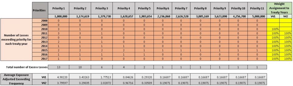
First, we divide the layer limit into equal size chunks called priorities (You may split by a log scale as done in the given example). Second, we determine the number of claims exceeding each priority for each historical treaty year. (This is similar to assuming a large loss threshold and selecting number of claims above it for each treaty year to determine claim frequency with the traditional method). Then average exposure adjusted exceeding frequency for each priority is calculated with some weight assignment. In the example, two weight options have been given to choose from. For example, weight W1 gives equal weight to each historical treaty year whereas weight W2 discards the oldest treaty year giving equal weights to the rest of historical treaty years.
The following table shows how the layer starting from the deductible of 1m to the end (i.e. limit + deductible) of 5m has been split into 11 priorities. For each priority number of claims above the priority for each historical treaty year has been determined. Then using weight assignments, average exceeding frequency for each priority has been determined. The premium has been used as the exposure base for exceeding frequencies.
The following formula shows the link between priorities, exceeding frequencies and alpha parameter (Please refer to Reference [1] for formulas used in this article).
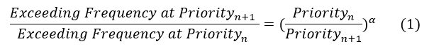
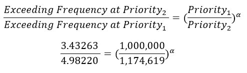
With average exceeding frequency being worked out for priorities n and n+1, the corresponding Pareto parameter alpha (α) can easily be determined using the above formula. For example, average exceeding frequencies given by weight W1 at priorities 1 and 2 can be used to determine the corresponding alpha as given below.
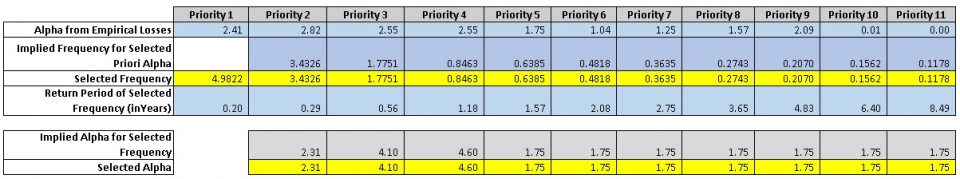
Generally, for priorities with credible enough historical claims working out alpha should be trivial. Alternatively, for a selected alpha exceedance frequency of the next priority can be determined. In the example, we used exceeding frequencies to work out alphas for lower priorities, whereas for higher priorities we used alphas to work out exceeding frequencies for the reason given below.
For priorities with a very few or no claims, the formula – (1) can be used to extrapolate with a selected alpha. This is especially applicable to higher layers with limited number of or no claims. The parameter invariability feature of Pareto distribution mentioned earlier applies here. Generally, we can use a benchmark alpha to work out exceeding frequency. In the example, we used the same alpha, which is in line with Industry benchmark for this particular class of business, from priority 5 onwards to extrapolate due to lack of historical experience with these priorities.
The following table shows exceeding frequency and alpha selection for each priority. In addition, alphas determined with Maximum Likelihood (MLE) method on historical claims are given, which can also be useful as a reference for the selection of alphas. The selections are highlighted in yellow.
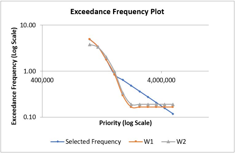
The log-log scale graph below shows selected average exceedance frequencies and that given by weight options. The selected exceedance frequencies follow that given by weight W1 up to priority 4. From priorities 5 to 9, the selections have been higher than that given by weight options. This indicates the expectation of higher claims frequencies than what has been observed in the past for these priorities. For priority 11, return period given by two weight options range from 1 in 5 years to 1 in 6 years. The exceedance frequency for the same priority corresponding to alpha selection provides a return period of 1 in 8.5 years indicating extrapolation with the same alpha provides a more optimistic view on return period.
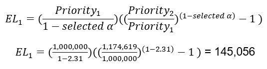
Next, the Expected Loss (EL) or severity between priorities n and n+1 can be determined with the following formula.
For example, EL between priorities 1 and 2 is given as follows.
Finally, the pure premium or risk premium between priorities n and n+1 can easily be worked out with the general frequency and severity based formula.

Above steps should be repeated for all priorities and risk premium for the layer is then given by summing up risk premium for each priority.
The following table shows Expected Loss and Risk Premium calculation for each priority with selected exceeding frequencies and alphas.

As a comparison we calculated the risk premium using the traditional method of fitting a single distribution. We fitted a single Pareto distribution with an alpha value of 1.76 on historical claims. The risk premium from the traditional method is 25% higher than that given by piecewise Pareto distribution. Such a price difference can easily put a reinsurer out of a quoting market signifying the importance of achieving reasonable pricing.
Advantages of the approach with piecewise Pareto distribution
- Provide great flexibility in pricing especially for higher layers where experience is sparse.
- Can take advantage of features such as parameter invariability of Pareto distribution for extrapolation.
- Easier to calculate expected values and variances.
- Can easily be programmed into a function or make it formula based in Excel for use.
- Can take advantage of benchmark alphas for pricing of higher layers.
However, there are certain disadvantages with Pareto distribution [1] that also applies to the approach described.
- The threshold should be above zero. It is not possible to use Pareto distribution for some proportional, stop loss and multiline treaties for which losses starting from zero is important.
- There are real-life loss distributions in which medium size losses are more probable than small or large losses. Distribution functions of such distributions have a turning or inflection point. Pareto distribution does not contain an inflection point.
Conclusion
This article looks at how piecewise Pareto distribution can be used for treaty pricing in P&C reinsurance over traditional method of using a single fitted distribution. The method takes advantage of some of the important features of Pareto distribution, provides great flexibility in fitting curves and allows underwriters and actuaries to take a pragmatic approach to pricing.
References
-
Swiss Re paper – “The Pareto model in property reinsurance – Formulas and applications” – by Markus Schmutz and Richard R. Doerr
-
“Reinventing Pareto: Fits for both small and large losses” – by Michael Fackler (http://www.actuaries.org/ASTIN/Colloquia/Hague/Papers/Fackler.pdf)
Special Note: The author would like to thank Mudit Gupta (FIAA), Australia and Frederic Boulliung (FSAS), Singapore for their invaluable feedback to improve the content of this article.
CPD: Actuaries Institute Members can claim two CPD points for every hour of reading articles on Actuaries Digital.