Pricing tree structures with shifting parameters

This article is a very brief summary of a full paper published in the ASTIN Bulletin, and presented to an Insights session in November 2017.  For reasons of copyright, the paper cannot be reproduced, but a pre-print can be found here, and the presentation here. Space limitations restrict the amount of detail in this article – see the full paper for further information.

Motivation

As a motivational example, consider the ANZSIC occupational classification.  It follows a tree (equivalently, hierarchical) structure, a small excerpt of which appears in Figure 1.  Here, A and B are the highest-level occupational groupings, and A1 to B8 are sub-groupings, as follows:

• A = Agriculture, Forestry and Fishing
  – A1 = Agriculture
  – A2 = Aquaculture
• B = Mining
  – B6 = Coal mining
  – B7 = Oil and gas extraction
  – B8 = Metal ore mining

In fact, the ANZSIC classification is much more extensive.  The highest level contains primary groupings $$A-S$$, and sub-groupings go to another four levels, e.g. $$K6322$$ = General insurance.

Now suppose that each node of the tree carries a risk parameter.  This could be one of any number of things but, in a pricing context, it might be expected claim cost per unit exposure.  As an example, workers compensation is sometimes priced at the nodes. 

There are two difficulties in the estimation of the parameters:

• Sample sizes of claims experience will often be small at the lower nodes of the tree;
• The parameters may shift over time.

Figure 1  ANZSIC hierarchy (excerpt)

Model

To establish a model of the risk parameters at the tree nodes, one thinks of any such parameter as a displacement from its parent’s parameter (actually, the full paper makes a somewhat more general allowance).  Thus, working down the General Insurance branch of the hierarchy, $$\beta_{K6} = \beta_{K} + \zeta_{K6}$$ where $$\beta_{K}$$ is the parameter at node $$K, \, \beta_{K6}$$ is the parameter at node $$K6$$, and $$\zeta_{K6}$$ is the displacement, assumed random with mean zero and normally distributed with known variance.  Similarly, $$\beta_{K63} = \beta_{K6} + \zeta_{K63} = \beta_{K} + \zeta_{K6} + \zeta_{K63}$$.

Observations, e.g. claim frequencies per unit exposure, are made at the lowest-level nodes of the tree (leaves), such as $$K6322$$.  Each of these observations is assumed to be a random variable with mean equal to the $$\beta$$ parameter at its leaf (e.g.  $$\beta_{K6322}$$). Again, the paper is more general.

This is a hierarchical model, and the problem of estimating its parameters was solved long ago (Taylor, 1979; Sundt, 1979,1980), provided that the parameters remained fixed over time.  The solution made use of credibility theory, in which case the model was a hierarchical credibility model, strictly a static form of such a model.

In practice, there are often many reasons why these parameters do change over time, in which case inclusion of such variation in the model is necessary.  Hence, the above model is converted to the following form, allowing the parameters to evolve over time:

$$\beta_{K6}^{t} = \beta_{K}^{t-1} + \zeta_{K6}^{t}$$

where the superscript denotes time.  Each parameter is now displaced from its parent’s parameter value at the preceding point of time.  The displacement is equivalent to the sum of two components, one equal to $$\zeta_{K6}$$  above, and another representing a further displacement due to the passage of time.  This is an evolutionary hierarchical credibility model.

Pricing procedure

There is a ready-made statistical procedure for estimation of parameters in an evolutionary model of the type described.  This is the Kalman filter (Harvey, 1989).  This accommodates a model:

• whose parameters evolve stochastically over time in a linear manner;
• whose observations are random variables with means depending linearly on the parameters;
• all of whose random variables are normally distributed.

Parameter estimation follows a procedure that is well-defined and straightforward, though requiring a substantial amount of matrix manipulation.  Variances and covariances of parameter estimates are also provided as part of the estimation process.

In the case of a large tree, such as that of ANZSIC codes, considerable organizational effort is required to ensure that the structure is correctly represented in the filter’s matrices.  The paper gives details of the book-keeping required to achieve this organization.

It is important to note that, since experience at each node is viewed as a displacement from its parent’s experience, estimation at the node will be affected by estimation at the parent node, and therefore, to some extent by all other nodes in the hierarchy.

Example

The paper provides a toy example, involving a hierarchy consisting of just 3 levels, with a total of 10 leaves.  Claim frequency per unit exposure is observed at each leaf.  The hierarchy parameters are selected over three periods, some parameters remaining static and others following defined trends.  Observations at the leaves are simulated according to the parameters there.

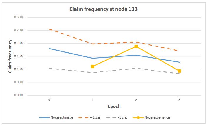
The Kalman filter is then applied to obtain parameter estimates, which can be compared with the known (but hidden) parameters.  Figure 2 gives an example for one leaf of the hierarchy.  The claims experience here is relatively small, and therefore volatile.  Its true claim frequency is flat over the three periods, at 0.18.

The figure plots the volatile experience for the three periods, and also the parameter estimates, together with a $$\pm 1 \times$$ standard error envelope.  The observations are seen to lie within the confidence envelope.

The filter smooths the series of observations considerably. This demonstrates the filter pooling experience over time and nodes to improve estimation. Over the three periods, the estimated claim frequency falls from its initial value of 0.18 to about 0.13, even though the underlying frequency has remained constant at 0.18.  This results mainly from reductions in experience at node 13.

Figure 2  Example of parameter estimation

Acknowledgments

This research was supported by a grant from the Actuaries Institute, and was also supported under Australian Research Council’s Linkage Projects funding scheme (project number LP130100723).

CPD: Actuaries Institute Members can claim two CPD points for every hour of reading articles on Actuaries Digital.

References

Harvey A C (1989). Forecasting, structural time series and the Kalman filter. Cambridge University Press, Cambridge, UK.
Sundt B (1979). A hierarchical credibility regression model. Scandinavian Actuarial Journal, 107-114.
Sundt B (1980). A multi-level hierarchical credibility regression model. Scandinavian Actuarial Journal, 25-32.
Taylor G C (1979). Credibility analysis of a general hierarchical model, Scandinavian Actuarial Journal, 1979(1), 1-12.