Gauss, Least Squares, and the Missing Planet
The field of statistics has a very rich and colourful history with plenty of interesting stories. Milton Lim describes his personal favourite – Carl Friedrich Gauss’ discovery of the method of least squares and the normal distribution to solve a particularly thorny problem in astronomy. So where did the ubiquitous bell curve originate from?
“It is not knowledge, but the act of learning, not possession, but the act of getting there, which grants the greatest enjoyment.”
– Carl Friedrich Gauss
|
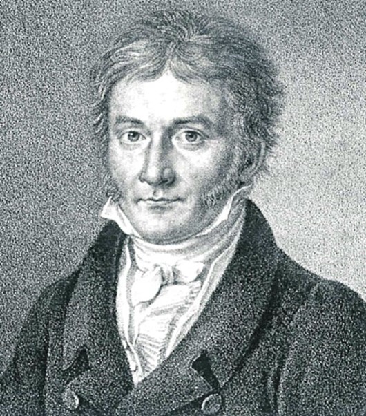
Figure 1: Carl Friedrich Gauss (1777 – 1855) as a young man. |
There is no doubt that Gauss was one of the geniuses of his age. As the apocryphal story goes: At the age of seven, on Gauss’ first day of school, his maths teacher decided to discipline the class with a tedious maths problem to compute the sum 1+2+3+ …+99+100. Although the teacher planned to keep the class busy for an hour, Gauss immediately shouted out the correct answer to the puzzle. The young genius noticed the shortcut of pairing the numbers (1+100) + (2+99) + … (50+51) to give 50 pairs of 101 equalling 5050, which we now call an arithmetic series.
The early history of statistics can be traced back to 1795 when Carl Fredrich Gauss, at 18 years of age, invented the method of least squares and the normal distribution to study the position of stars and other celestial bodies subject to random measurement errors.
The ‘missing’ planet?
On 1 January 1801, the planetoid Ceres was discovered and tracked for 40 days before being lost in the glare of the Sun. This was an exciting discovery, as the Titius-Bode Law predicted a ‘missing’ planet between Mars and Jupiter. This law gave an approximate relationship between the size of the orbits of each planet to follow this simple formula:
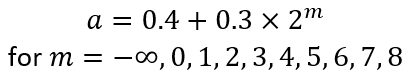
Where ‘a’ is the semi-major axis of each planet in terms of astronomical units (AU) i.e. distance from Earth to the Sun. For the outer planets (Jupiter onwards), the formula implies that the next planet is roughly twice as far from the Sun as the previous planet, as presented in the following table:
|
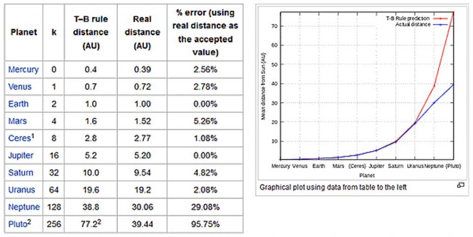
Figure 2: Actual vs Predicted with the Titius-Bode Law for the planets, which is fairly accurate from Mercury to Uranus The accuracy of this simple rule of thumb is mostly due to coincidence. |
The Ancient Greeks described planets as “wandering stars” because they appear to move against the background of fixed stars (which are so far away that they never appear to move). Johannes Kepler was mystified by the large gap between Mars and Jupiter. Ranyard (1892) describes that many people believed that “a planet formerly travelling along this seemingly vacant track had been destroyed as punishment from the Gods due to the wickedness of its inhabitants”.
By the early 19th Century, speculation about extra-terrestrial life on other planets was open to debate, and the potential new discovery of such a close neighbour to Earth was the buzz of the scientific community. In fact, this was the first detection of what is known today as the Asteroid Belt between Mars and Jupiter, of which Ceres is the largest object.
However, the position of Ceres was ‘lost’ a few months later after it re-emerged from the glare of the Sun, as astronomers could not extrapolate its position from the small amount of collected data. They needed to solve Kepler’s complex non-linear equations for elliptical orbits with data on less than 1% of the total orbit – a formidable mathematical challenge.
|
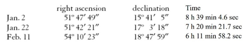
Figure 3: Extract of the raw data of 19 observations over 42 days of the newly discovered Ceres. |
A group of 24 prominent astronomers formed ‘The Society for the Detection of a Missing World’, who became fondly known as the ‘Celestial Police’ because they were charged to ‘arrest’ the missing planet. The French mathematician Pierre-Simon Laplace, another founder of probability theory, believed this problem was impossible to solve with such little data. Figure 3 shows the first, middle and last observations that Gauss used to maximise the range of the orbit and minimise the prediction error.
Law of Probable Errors
A key challenge is that the recorded data on Ceres was subject to error, which could accumulate into even more imprecise extrapolations if not allowed for properly. What is the best mathematical description of the random measurement errors between the planet’s true and observed positions? Gauss pondered this puzzle, and realised that the ‘law of probable errors’ must fulfil these three basic assumptions:
- Small errors are more likely than large errors;
- The likelihood of errors of magnitudes and x and -x are equal (the distribution is symmetrical); and
- When several measurements are taken of the same quantity, the average (arithmetic mean) is the most likely value.
Nowadays, the average is a standard and widely used measure but at the time it was not completely obvious and has had a controversial history. Stahl (2006) recounts “Astronomy was perhaps the first science that demanded accurate measurements, and hence plagued by the problem of several distinct observations of the same quantity. In the 2nd century BC, Hipparchus seems to have favoured the midrange. In the 2nd century AD, Ptolemy, faced with several discrepant estimates for the length of a year, decided to work with the observation that fit his theory best. By the 16th century period of Tycho Brahe and Johannes Kepler, astronomers devised their own, often ad hoc, methods for extracting a measure of central tendency out of their data. Sometimes they averaged, sometimes they used the median, sometimes they grouped their data and resorted to both averages and medians!”
|
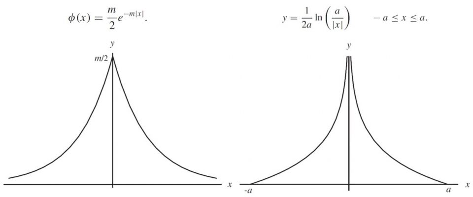
Figure 4: Laplace’s first (left) and second (right) Error Curves. |
In 1774, Laplace published his ‘First Law of Error’, using only the first two assumptions, he derived the Laplace (or double exponential) distribution. The Laplace distribution has the useful property of minimising the total absolute deviation from the median, but predicted too high a frequency or large errors. Only three short years later, he revised his attempt with his ‘Second Law of Error’. This was an even more disastrous attempt with an embarrassing infinite singularity at __ but only a finite domain of errors, which was clearly unrealistic.
|
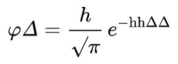
Figure 5: Gauss’ formula in his original notation |
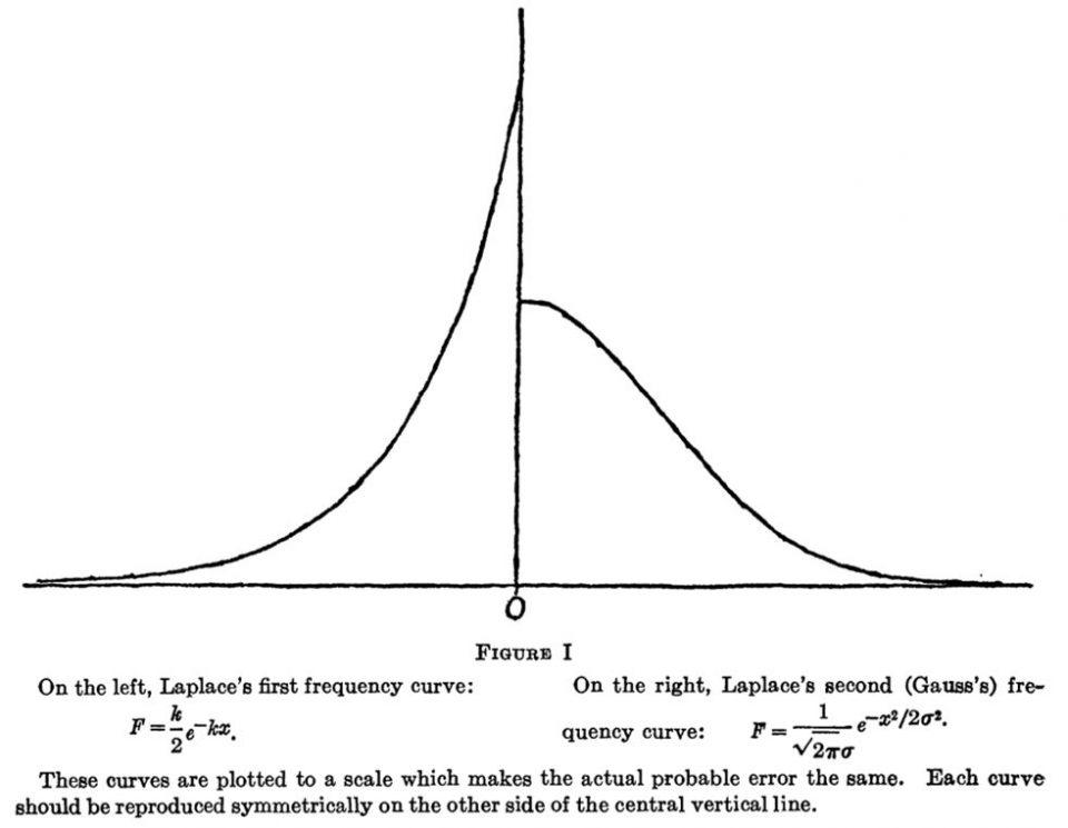
Gauss successfully derived his well-known ‘bell-curve’ distribution as the only solution that satisfies the three basic assumptions, with his original notation shown in Figure 5. Incidentally, Gauss coined the term ‘normal distribution’ to refer to the ‘normal equations’ of his work, which means orthogonal or perpendicular, rather than usual. Figure 6 contrasts the Laplace and Gaussian distributions, leading to a more realistic model of measurement errors that would eventually lead to the re-discovery of the missing Ceres.
|
Figure 6: Laplace vs Gaussian distributions. |
By 1810, Laplace proved the Central Limit Theorem, which states that estimates of the mean converge to a normal distribution around the true mean as data accumulates, cementing the theoretical foundation of the normal distribution. He justified this by imagining the error involved in an individual observation as the aggregate of many independent ‘elementary’ or ‘atomic’ errors. Examples of such errors might be the atmospheric turbulence that causes the twinkling of stars and the measurement crudeness of the early telescopes.
Even Sir Francis Galton praised this famous theorem, stating “I know of scarcely anything so apt to impress the imagination as the wonderful form of cosmic order expressed by the “Law of Frequency of Error”. The law would have been personified by the Greeks and deified, if they had known of it. It reigns with serenity and in complete self-effacement, amidst the wildest confusion. The huger the mob, and the greater the apparent anarchy, the more perfect is its sway. It is the supreme law of Unreason. Whenever a large sample of chaotic elements are taken in hand and marshalled in the order of their magnitude, an unsuspected and most beautiful form of regularity proves to have been latent all along.”
The English statistician Karl Pearson later popularised the term “normal distribution” and commented “Many years ago, I called the Laplace-Gaussian curve the normal curve, which name, while it avoids an international question of priority, has the disadvantage of leading people to believe that all other distributions of frequency are in on sense or another ‘abnormal’.” In 1782, Laplace was the first to calculate the value of the integral…
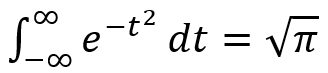
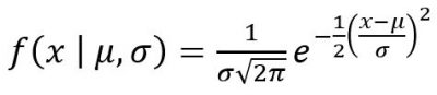
…to determine the normalisation constant to make the distribution sum to one. Later, in the early 1900’s, Pearson (inventor of the correlation coefficient) was the first to add the standard deviation σ as seen in modern notation. Shortly after in 1915, Sir Ronald Fisher (father of hypothesis testing) added the location parameter μ, to put the finishing touches on the immortalised formula:
The Prince of Mathematics
“An opinion had universally prevailed that a complete determination from observations embracing a short interval of time was impossible – an ill-founded opinion”.
– Carl Friedrich Gauss
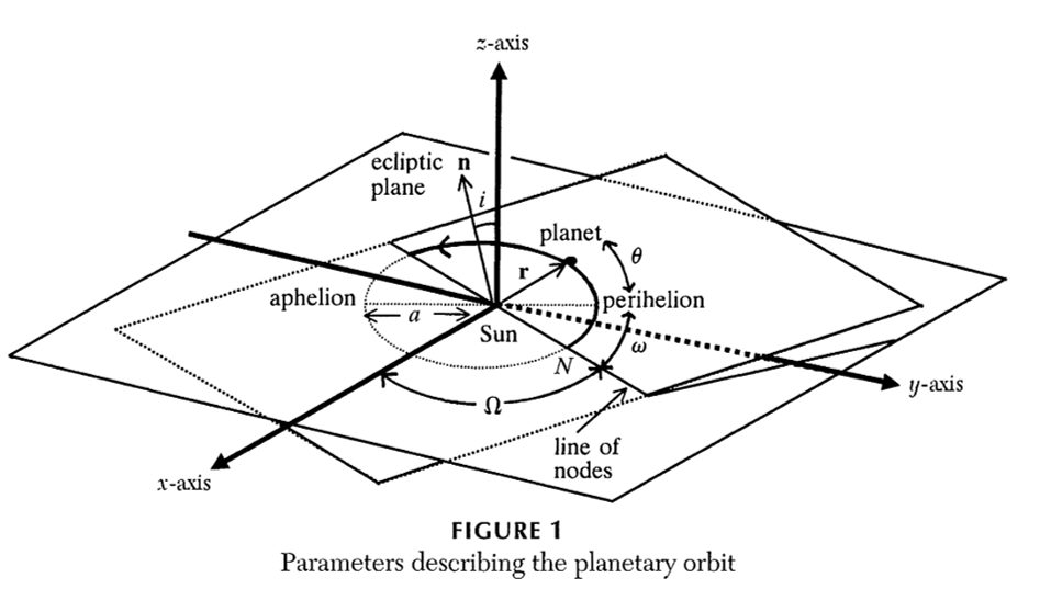
The 24-year-old Gauss tackled the orbit problem, assuming only Kepler’s three laws of planetary motion, with his newly discovered error distributions and his method of least squares for three months. He spent over 100 hours performing intensive calculations by hand without any mistakes (and without the luxury of today’s computers!). He had to estimate the six parameters of the orbit (as shown in Figure 7) from only 19 data points, subject to random measurement errors. He even invented new techniques such as the Fast Fourier Transform for interpolating trigonometric series, which produced efficient numerical approximations of the elliptical orbit. This is much earlier than Joseph Fourier’s 1825 results and the modern FFT algorithm by James Cooley and John Tukey in 1965, which has been described as “one of the most important numerical algorithms of our lifetime” by Heideman et al (1984). Teets & Whitehead (1999) and Tennenbaum & Director (1998) document the full mathematical details of Gauss’ work.
|
Figure 7: The orbit of Ceres is governed by six parameters: a,e,i,π,τ,Ω. |
His final calculations pointed astronomers to an entirely different region of the sky, previously overlooked by other scientists. He was the only person who successfully predicted the new position of the asteroid, to with a half-degree error, which allowed the asteroid to be ‘found’ again by astronomers. Gauss noted in his diary “This first application of the method (of least squares)… restored the fugitive (planet) to observation”. He later refined his method to be so efficient that it only required three data points and he could calculate the entire orbits of newly discovered comets in one hour, whereas older methods by Leonard Euler took three days of calculations. Even Laplace congratulated Gauss with “The Duke of Brunswick has discovered more in his country than a planet: a super-terrestrial spirit in a human body”.
In Gauss’ day, during the Age of Enlightenment, astronomy was considered a glamorous area of research, similar to how Artificial Intelligence is currently experiencing a boom in research efforts. But the 18th Century astronomy included the pseudo-scientific field of astrology (complete with star signs and horoscopes!) with most of the general public unable to distinguish between science fact and exaggerated fiction. This success catapulted him into fame in the academic world, where he was appointed Professor of Astronomy and Director of the Göttingen Observatory, launching one of the most fruitful careers in the history of science.
Arguably, Gauss could be considered as one of the world’s first data scientists, thanks to his solution to such a ‘wicked’ problem. Despite the complete lack of computing power, his mathematical ingenuity allowed him to devise powerful techniques for model fitting to the limited noisy data, to earning him the reputation as the “Prince of Mathematics”. As an ardent perfectionist, he was notorious for publishing only elegant proofs without any of his workings, justifying that “all traces of analysis must be suppressed for the sake of brevity”. Other mathematicians lamented that if he had published all his research while he was still alive, rather than posthumously, he would have sped the advance of the entire field of mathematics by at least 50 years.
|
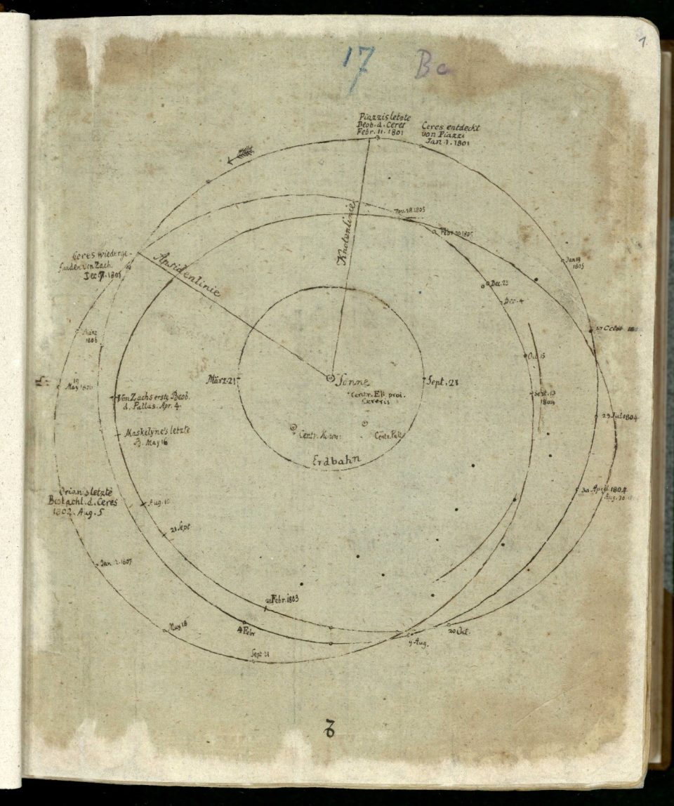
Figure 8: Gauss’ original sketch. |
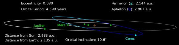
Figure 8 shows Guass’ original sketch of the orbits and the scarcity of the data (a geocentric arc of only three degrees, which is less than 1% of the orbit). Figure 9 shows the actual orbit of Ceres is moderately inclined (10.6°) to thee plane of the Solar System, the highest out of all the planets except Pluto, which added to the complexity of the prediction problem).
|
Figure 9: Actual orbit of Ceres. |
However, few great discoveries come without controversy. Based on historical evidence, the first publication of the method of least squares was due to the Frenchman Adrien Marie Legendre in 1805. However, Gauss did not officially publish his method until 1809 in his famous treatise “Theoria motus corporum coelestium in sectionibus conicis solem ambientum” (Theory of the Motion of the Heavenly Bodies Moving about the Sun in Conic Sections), where he claimed that he had been using this method since 1795. When Gauss first discovered this at 18 years of age, he considered the least squares method to be quite obvious to any mathematician and relatively inconsequential. As a result, he did not bother to publish this rather pragmatic method in applied maths, and instead he pursued deeper theoretical results in pure mathematics.
This sparked off one of the most famous priority disputes in mathematics (second only to the Newton vs Leibniz controversy over the invention of calculus). To complicate the matter, the American Robert Adrian also seemed to have independently discovered least squares in the context of survey measurements, but it is possible that he might have read Legendre’s 1805 work. Plackett (1972) and Stigler (1981) attempted to verify some of these priority claims. The moral of the story seems to be to always publish your work first!
Least Squares: a modern approach
The least squares approach to fitting lines and curves remains a mainstay in modern statistics. Stigler (1981) commented that “the method of least squares is the automobile of modern statistical analysis, despite its limitations, occasional accidents, and incidental pollution, it and its numerous variations, extensions, and related conveyances carry the bulk of statistical analyses, and are known and valued by nearly all.”.
At first glance, the problem appears to be solvable by marking the observations as data points on graph paper and drawing in a line of best fit. More formally, the least squares estimate involves finding the point closest from the data to the linear model by the “orthogonal projection” of the y vector onto the linear model space. I suspect that this was very likely the way that Gauss was thinking about the data when he invented the idea of least squares and proved the famous Gauss-Markov theorem in statistics.
While techniques continue to evolve, I suspect that Gauss would be very proud if he knew that his method of least squares is still a cornerstone of modern statistics and exciting new research is being done to build on and improve this fundamental technique within statistical machine learning theory. Figure 10 shows a series of diagrams to illustrate the evolution of our modern interpretation of the method of least squares.
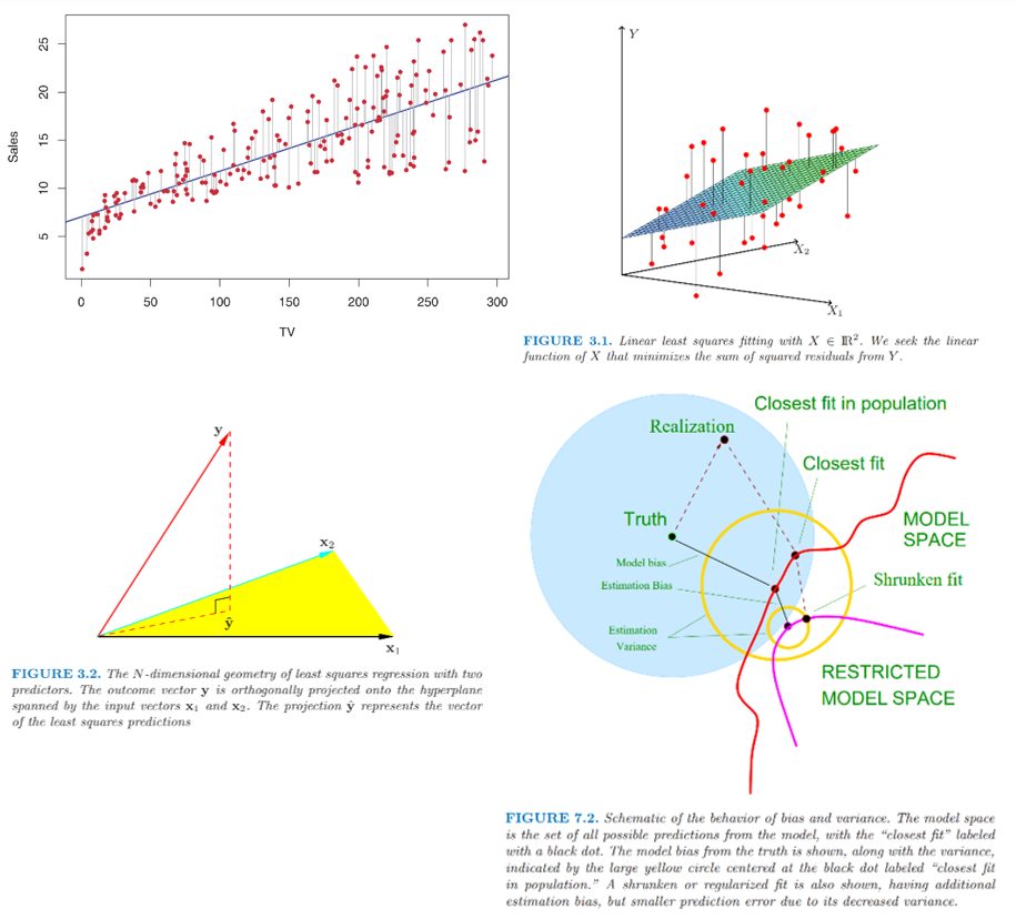
|
Figure 10: Different perspectives of least squares fitting |
Epilogue
Gauss revealed his philosophy of learning and pursuit of knowledge, which many readers may relate to. “It is not knowledge, but the act of learning, not possession but the act of getting there, which grants the greatest enjoyment. When I have clarified and exhausted a subject, then I turn away from it, in order to go into darkness again. The never-satisfied man is so strange; if he has completed a structure, then it is not in order to dwell in it peacefully, but in order to begin another. I imagine the world conqueror must feel thus, who, after one kingdom is scarcely conquered, stretches out his arms for others.”
This passion for discovery and learning is evidenced by his work beyond pure mathematics. In his 70s, Gauss also dabbled in actuarial work. The University of Göttingen’s Pension Fund for the Professor’s Widows became worried about the increasing number of claiming widows threatening the long-term solvency of the fund. They approached Gauss, who applied his mathematical wizardry to build an actuarial model of the pension fund for both income (e.g. contributions from existing employees, investment returns) and expenses (pension payments, number of current widows and expected number of future widows), utilising past and projected mortality, demographic and financial market data. As recounted in Read (2016), his work reformed the Widow Fund onto a sound actuarial basis, which allowed the University to surprisingly increase the pension payments to widows by forecasting the expected increase in the number of professors and restricting their conditions for beneficiaries.
Using his financial acumen, Gauss later made shrewd investments in under-valued corporate bonds issued by private companies. He made a small fortune in the last four years before his death: his humble professor’s salary was only 1,000 thalers per year, yet his estate totalled 170,000 thalers (equivalent to $AUD 34 million in today’s dollars!). His prolific career included being a 19th Century mathematician, physicist, astronomer, statistician, data scientist, life insurance / pensions actuary and a very profitable investor!
Gauss ushered in an age where scientists used sophisticated mathematics to find things that were invisible to the naked eye. For example, both Neptune and Pluto were discovered in 1846 and 1930 respectively, by mathematical predictions (i.e. data science!) due to their gravity causing “wobbling” in the observable orbits of neighbouring planets.
Since Gauss’s cryptic entry of “meine Methode” in his mathematical diary on 17 June 1798, his humble discovery of least squares and the normal distribution has permeated almost every branch of science, forming the bedrock of mathematical statistics and the powering today’s era of machine learning and artificial intelligence. Hopefully this little history lesson might help us to appreciate the simple yet powerful tool of linear regression in the context of data science, the art and science of extracting useful insights from data.
|
References Adrain, R. (1808), “Research concerning the probabilities of the errors which happen in making observations”, Analyst Gauss, C.F. (1809), “Theory of Motion of the Heavenly Bodies Moving about the Sun in Conic Sections”, Hamburg, Perthes et Besser Hastie, T., Tibshirani, R., & Friedman, J. (2009), “The Elements of Statistical Learning: Data Mining, Inference, and Prediction” Springer Heideman, M.T., Johnson, D.H. & Burrus, C.S. (1984), “Gauss and the History of the Fast Fourier Transform”, IEEE ASSP Magazine Kuppers, M. et al (2014) “Localised sources of water vapour on dwarf planet Ceres”, Nature Plackett, R.L. (1972) “The discovery of the method of least squares”, Biometrika, 59(2) pp 239-251 Ranyard, A. (1892) “Old and New Astronomy”, Longmans Green & Co. Read, C. (2016) “The Econometricians: Gauss, Galton, Pearson, Fisher, Hotelling, Cowles, Frisch, Haavelmo”, Palgrave Macmillan Stahl, S. (2006) “The Evolution of the Normal Distribution”, Mathematics Magazine, 79 pp. 96-113 Stigler, S. (1981) “Gauss and the Invention of Least Squares”, Annals of Statistics, 9 (3), pp. 465-474 Teets D. & Whitehead K. (1999), “The Discovery of Ceres: How Gauss Became Famous”, Mathematics Magazine, 72 (2) pp. 83-93 Tennenbaum, J. & Director, B. (1998), “How Gauss Determined the Orbit of Ceres” Weiss, L. (1999), “Gauss and Ceres”, Rutgers University Wilson, E.B. (1923), “First and Second Laws of Error”, Journal of the American Statistical Association, 18 (143) pp. 841-851 |
CPD: Actuaries Institute Members can claim two CPD points for every hour of reading articles on Actuaries Digital.