Pricing without Data – Piecewise Pareto Distribution for Exposure based Treaty Pricing

Typically, non-proportional treaty pricing in P&C reinsurance is performed with well-known loss frequency and severity-based approaches using historical experience. When historical experience is sparse or no longer applicable, or when it is a new treaty, underwriters and actuaries tend to use the traditional exposure based pricing method with exposure curves. A common practice is to use one exposure curve across the risk profile and in some cases different exposure curves for different risk bands of the risk profile of the class of business. Therefore, there is little flexibility associated with this traditional method.

We introduced a piecewise Pareto distribution based method, which is not new to reinsurance pricing and based on mathematics related to Pareto distribution given in a Swiss Re paper [1], for experience based treaty pricing in a previous article. In fact, we can extend the same method for exposure based pricing. In this article we discuss how the piecewise Pareto distribution based method can be used for non-proportional treaty pricing with exposure curves to provide greater flexibility and allow underwriters and actuaries to take a pragmatic approach to pricing, which can lead to better pricing outcomes for reinsurers.

2. Traditional exposure based pricing

The traditional exposure based pricing involves a risk profile (i.e. distribution of risks insured under different sum insured bands) and a loss ratio of the class of business associated with the treaty being priced and exposure curves (Refer to [4] for the definition) to determine risk premium applicable to the non-proportional layer. Some of the widely used exposure curves in reinsurance are Swiss Re curves, Munich Re curves and Lloyds curves to name a few. There is a plethora of literature available on exposure based pricing if a reader is interested in exploring the details of how pricing is performed with the exposure based method (Refer to [4] for a comprehensive introduction).

Exposure based pricing has its own drawbacks. The following are several of them.

• Market based exposure curves are most likely to be used raising the issue of appropriateness of these curves to reflect underlying risks.
• Market curves are based on historical data. Some of the curves being used have a history of 20 to 30 years. They do not allow for new claim types (e.g. property damage due to cyber).
• Only allow to determine risk premium. There is no volatility element typically required for loading with technical pricing.
• There is no indication of return periods of losses unless frequencies are worked out explicitly.
• Apart from the selection of different exposure curves for different risk bands there is no flexibility allowed with pricing.
• For exposure based pricing to work risk profiles should be given on per location basis. Often risk profiles are not given in this format thus impacting pricing. This issue equally applies to both exposure based method and piecewise Pareto based method we are introducing.

In the next section of the article we discuss how the piecewise Pareto distribution based method can be used to address some of these issues.

3. Exposure based pricing with piecewise Pareto distribution

It is best to use an example to explain how a piecewise Pareto distribution can be used with exposure based pricing. We considered a property class of business with small to medium sized commercial risks applied on a non-proportional treaty layer with a limit of USD 4 million in excess of a deductible of USD 1 million (i.e. USD 4m xs 1m). We chose Swiss Re-Y2 exposure curve [4], which represents small scale commercial risks on Total Sum Insured (TSI) value basis to apply across all risk bands of the risk profile of the class of business (Risk profile is given in Table 2). We assumed that underlying risks are relatively homogeneous and therefore, the selected curve is appropriate to represent these underlying risks. The non-catastrophe loss ratio for the class of business is assumed to be 75%.

3.1. Deriving exceedance frequencies from exposure curves

First, we divided the layer from the deductible of USD 1 million to the end of USD 5 million (deductible + limit) into equal size chunks called “priorities” (It may split by using a log scale as done in Table 1 for this example). Next, we derived exceeding frequency for each priority with the selected exposure curve, Swiss Re-Y2. To derive exceeding frequencies we followed the steps given below.

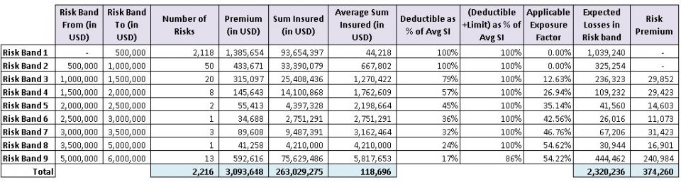
1: For each risk band given in Table 2 derive risk premium between priorities n and n+1 with the selected exposure curve using the traditional exposure based pricing method.

Risk premium for a risk band is given by:

For example, the risk premium of risk band 4 between priorities 1 and 2 is given by:

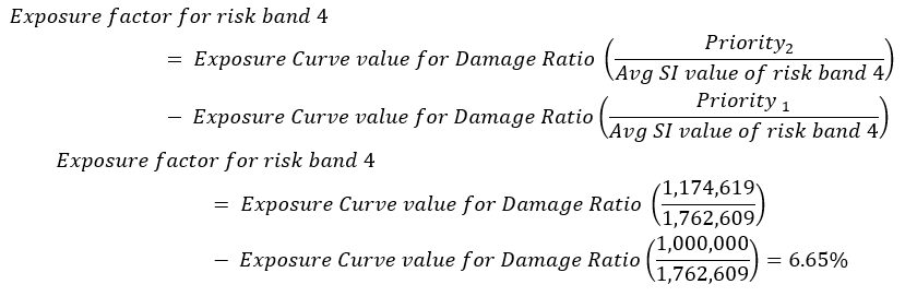
The Exposure factor comes from exposure curve values corresponding to damage ratios at priorities n and n+1 as given below:

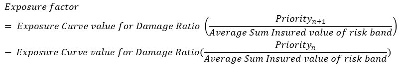
For example, the Exposure factor for risk band 4 between priorities 1 and 2 is given by:

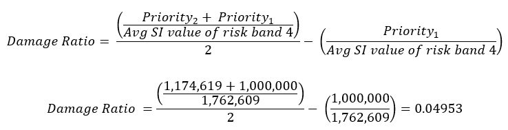
2: For each risk band derive the average damage ratio applicable to the part of layer limit between priorities n and n+1. We have taken the average between the two priorities to determine the damage ratio. Therefore, for a risk band the damage ratio is given by:

For example, the damage ratio of risk band 4 between priorities 1 and 2 is given by

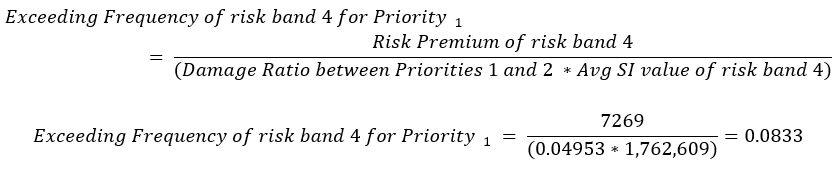
3: For each risk band derive exceeding frequency for priority n. The exceeding frequency for a risk band can be derived with the loss frequency and severity based formula as given below.

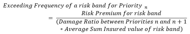
For example, the exceedance frequency of risk band 4 for priority 1 is given by

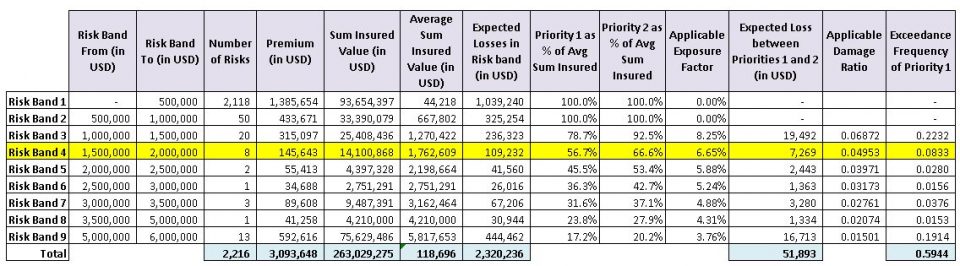
4: Then the exceeding frequency for priority n is given by summing up exceedance frequency from each risk band. For example, the exceeding frequency for priority 1 from all applicable risk bands is 0.5944 as given in Table 2.

5: Repeat steps 1 to 4 for each priority.

Table 2 below shows the exceeding frequency of each risk band at priority 1 derived with above steps. The calculations given in steps 1 to 4 for risk band 4 are highlighted in yellow. Exceeding frequencies derived for other priorities are given in the next section in Table 3.

Once exceedance frequencies have been derived for priorities we can use the piecewise Pareto distribution based method to determine risk premium for the layer with the well-known loss frequency and severity based approach. We have observed that some of the commercial Dynamic Financial Analysis (DFA) tools tend to use a similar approach to what we have described above with exposure curves and risk profiles for simulations. These tools work out loss frequencies and severities based on damage ratios from exposure curves, and average sum insured values and risk premiums.

It is important to highlight that there is a disparity in how loss severities are represented with piecewise Pareto distribution and selected exposure curve based methods. In the example, loss severities from the selected exposure curve, Swiss Re-Y2 are based on an MBBEFD distribution [3] whereas with the method we introduced loss severities come from Pareto distributions. This disparity can lead to a significant deviation in risk premium. Despite such a disparity we can still use above exceeding frequencies to form a view on return periods of expected losses and use them with benchmark alpha parameter values of Pareto distribution particularly for higher priorities to derive risk premiums. We believe the flexibility piecewise Pareto distribution based method provides compared to the traditional exposure based pricing outweighs any drawback that may arise from this disparity.

3.2: Risk premium calculation with piecewise Pareto distribution

In this section we describe how exceedance frequencies can be used with piecewise Pareto distributions to determine risk premium of the layer.

3.2.1: Pareto parameters from exposure curve based exceedance frequencies

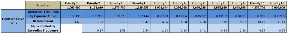
As we mentioned earlier exceeding frequencies derived from exposure curves can be used as a basis to determine risk premium with the piecewise Pareto distribution based method. The following table shows exceedance frequencies derived with the selected exposure curve and alpha parameter values of piecewise Pareto distribution corresponding to these exceedance frequencies (Pareto distribution has two parameters – scale or threshold and shape often denoted as alpha, α).

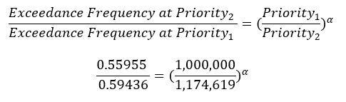
The following formula shows the link between priorities, exceeding frequencies and alpha parameter values (Refer to Reference [1] for formulas used in this section).

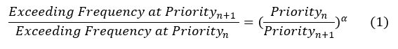
For example, exceeding frequencies at priorities 1 and 2 can be used to derive the corresponding alpha parameter value as given below.

As can be seen alpha parameter values vary across priorities particularly for higher priorities. Alpha parameter values at higher priorities are well below the market benchmark range of 1.8 to 2.5 we would expect for this particular class of business with small to medium sized commercial risks. This raises the question of appropriateness of the selected exposure curve for higher risk bands.

3.2.2: Selection of exceeding frequencies and Pareto parameters

Next, we selected exceeding frequencies taking the risk profile and market benchmarks of alpha parameter values into consideration. Accordingly, selected exceedance frequencies and alpha parameter values are given in the table below. The selections are highlighted in yellow.

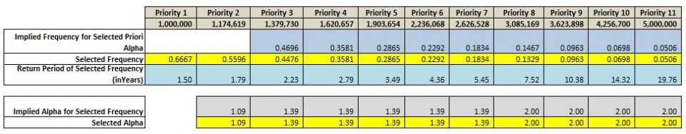
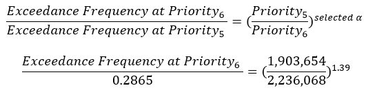
With priorities 1 to 3 and 8, alpha parameter values are based on selected exceedance frequencies using formula (1) similar to what we have shown above for exceedance frequencies with the selected exposure curve. From priority 4 onwards (except priority 8) we have used selected alpha parameter values to determine exceedance frequencies still using the formula (1). For example, the exceedance frequency for priority 6 is given by:

As can be seen the selections are largely kept the same as implied except the exceeding frequency at priorities 1 to 3 and 8. However, in practice, underwriters and pricing actuaries have the flexibility of selecting exceedance frequencies and alpha parameter values based on what they perceive as reasonable for the risk profile and the class of business.

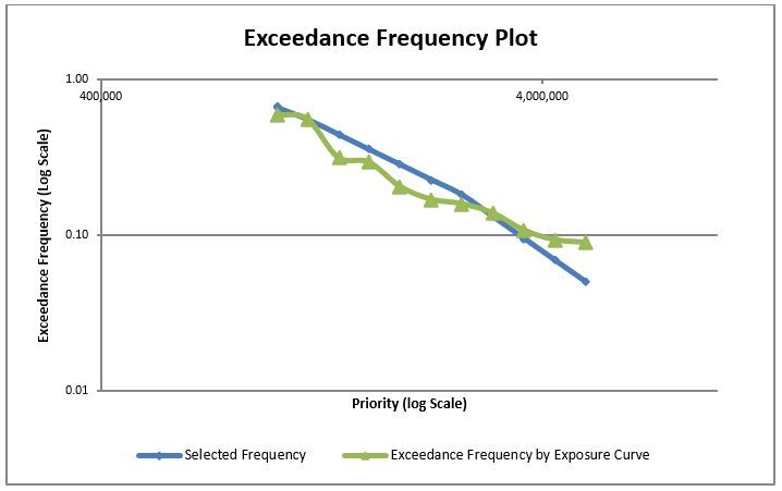
We assumed that for lower priorities from priority 1 to 7 exceedance frequencies are slightly higher than that given by the selected exposure curve. Then we adopted a benchmark alpha parameter value of 2 representing small to medium sized commercial risks from priority 8 onwards. We assumed that losses in priorities 10 and 11 have a return period in the range 15 to 20 years. For the assumption on return period, we considered the number of risks in risk bands that can result in losses to priorities 10 and 11. As a reasonableness check the return period of losses of similar magnitude from other similar portfolios can be compared. The exceedance frequency at priority 11 has a return period of almost 1 in 20 years from our selection compared to a return period of 1 in 11 years given by the selected exposure curve. Thus, we have a more conservative selection of exceedance frequencies at lower priorities and a more optimistic selection at higher priorities. The log-log scale graph below shows selected exceedance frequencies (blue line) and that given by the selected exposure curve (green line). The log-log plot is useful with the selection process as we expect straight line segments with the selected exceeding frequencies and alpha parameter values.

3.2.3: Risk premium calculation

Next, expected loss or severity between priorities n and n+1 can be determined with the following formula.

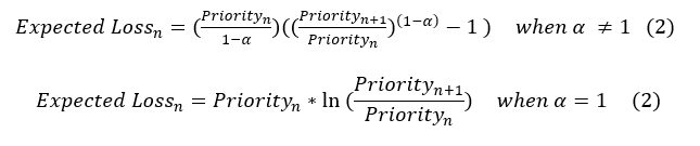
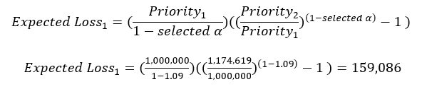
For example, the expected loss between priorities 1 and 2 with the selected alpha parameter value is given as follows.

Finally, pure premium or risk premium between priorities n and n+1 can easily be worked out with the general loss frequency and severity based formula.

Above steps should be repeated for all priorities and risk premium for the layer is then given by summing up risk premium for each priority. The following table shows expected loss and risk premium for each priority with selected exceeding frequencies and alpha parameter values given in Table 4.

4: Comparison of results between traditional exposure based and piecewise Pareto distribution based methods

We compared risk premium calculated with the traditional exposure based method and the piecewise Pareto distribution based method, which includes two approaches, exceedance frequencies derived from the selected exposure curve and selected exceedance frequencies and alpha parameter values.

To determine risk premium with the traditional exposure based method, we followed the step 1 given in the Section 3.1 for each risk band between the deductible and the layer limit. The following table shows risk premium derived for the layer.

To derive risk premium with exceedance frequencies from the selected exposure curve and derived alpha parameter values, a reader needs to follow steps given in the Section 3.2.3 with exceedance frequencies and alpha parameter values given in Table 3.

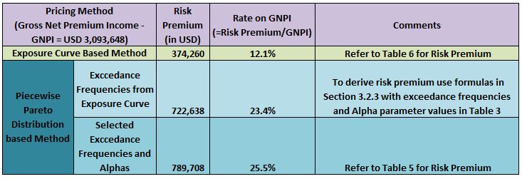
The results clearly show a significant deviation between the traditional exposure based and piecewise Pareto distribution based methods. As mentioned earlier the disparity in loss severity represented by these two methods attributes to this deviation. As an additional measure, the Rate on GNPI can be compared with that of other similar treaties to assess the reasonableness of the approach we have taken to pricing.

5: Advantages of the approach with piecewise Pareto distribution

• Provide great flexibility with pricing compared to the traditional exposure based method particularly for pricing of higher layers.
• Can take advantage of features such as parameter invariability of Pareto distribution [2] for extrapolation into higher layers.
• Easier to calculate expected values and variances. With pricing, variances can be used for loading on volatility. This is not possible with the traditional exposure based method.
• Can take advantage of benchmark alpha parameters particularly for pricing of higher layers.
• Can be used as an additional source to compare against experience based pricing.

However, there are certain disadvantages with Pareto distribution [1] that also applies to the method described in the article.

• The threshold should be above zero. It is not possible to use Pareto distribution for some proportional, stop loss and multiline treaties for which losses starting from zero is important.
• There are real-life loss distributions in which medium size losses are more probable than small or large losses. Distribution functions of such distributions have a turning or inflection point. Pareto distribution does not contain an inflection point.

Conclusion

The traditional exposure based method is a relatively simple approach to pricing with limited flexibility. The piecewise Pareto distribution based method described in this article allows us to leverage on the traditional exposure based method, utilise market benchmarks for alpha parameter values, and provides the opportunity to exercise better judgement. Moreover, this method takes advantage of some of the important features of Pareto distribution. Therefore, the piecewise Pareto distribution based method provides greater flexibility and allows underwriters and actuaries to take a more pragmatic approach to pricing compared to the traditional exposure based pricing.

References

1. Swiss Re paper – “The Pareto model in property reinsurance – Formulas and applications” – by Markus Schmutz and Richard R. Doerr, 1998.
2. “Reinventing Pareto: Fits for both small and large losses” – by Michael Fackler (http://www.actuaries.org/ASTIN/Colloquia/Hague/Papers/Fackler.pdf)
3. “The Swiss Re Exposure Curves and the MBBEFD Distribution Class” – by Stefan Bernegger (https://www.casact.org/library/astin/vol27no1/99.pdf)
4. Swiss Re paper – “Exposure Rating” by Daniel Guggisberg UP, 2004

Further Readings

1. “Introduction to Exposure Rating” – by Markus Gesmann, May 2015 (https://mran.microsoft.com/snapshot/2015-09-06/web/packages/mbbefd/vignettes/Introduction_to_Exposure_Rating.pdf)

Special Note: The author would like to thank Mudit Gupta (FIAA), Australia and Frederic Boulliung (FSAS), Singapore for their invaluable feedback to improve the content of this article.

CPD: Actuaries Institute Members can claim two CPD points for every hour of reading articles on Actuaries Digital.